openmaterials.ai / codes / pycalphad
pycalphad: CALPHAD Gibbs energy models and equilibria in Python
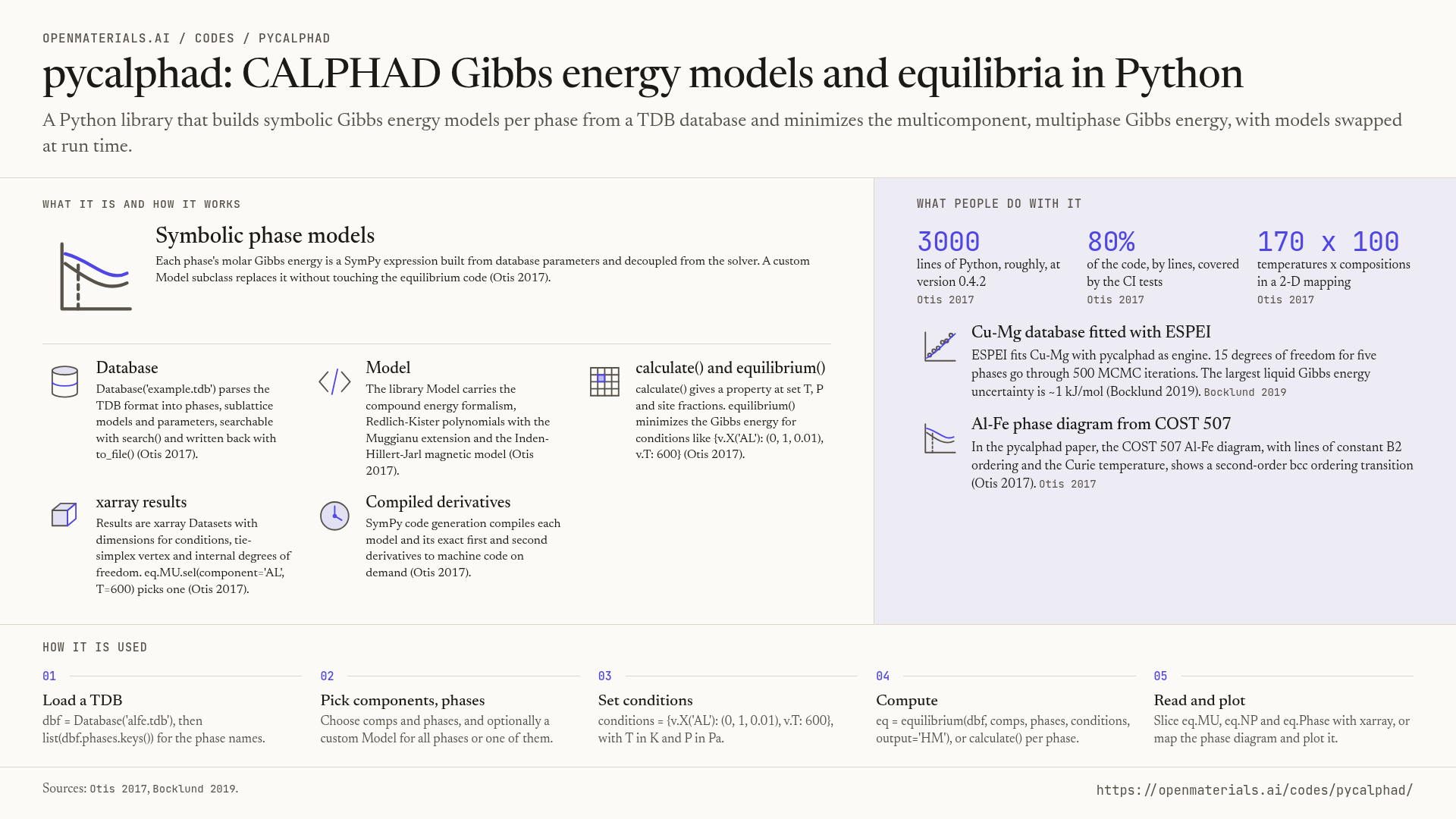
A Python library that builds symbolic Gibbs energy models per phase from a TDB database and minimizes the multicomponent, multiphase Gibbs energy, with models swapped at run time.
What it is and how it works
Symbolic phase models
Each phase's molar Gibbs energy is a SymPy expression built from database parameters and decoupled from the solver. A custom Model subclass replaces it without touching the equilibrium code (Otis 2017).
Database
Database('example.tdb') parses the TDB format into phases, sublattice models and parameters, searchable with search() and written back with to_file() (Otis 2017).
Model
The library Model carries the compound energy formalism, Redlich-Kister polynomials with the Muggianu extension and the Inden-Hillert-Jarl magnetic model (Otis 2017).
calculate() and equilibrium()
calculate() gives a property at set T, P and site fractions. equilibrium() minimizes the Gibbs energy for conditions like {v.X('AL'): (0, 1, 0.01), v.T: 600} (Otis 2017).
xarray results
Results are xarray Datasets with dimensions for conditions, tie-simplex vertex and internal degrees of freedom. eq.MU.sel(component='AL', T=600) picks one (Otis 2017).
Compiled derivatives
SymPy code generation compiles each model and its exact first and second derivatives to machine code on demand (Otis 2017).
What people do with it
- 3000lines of Python, roughly, at version 0.4.2Otis 2017
- 80%of the code, by lines, covered by the CI testsOtis 2017
- 170 x 100temperatures x compositions in a 2-D mappingOtis 2017
Cu-Mg database fitted with ESPEI
ESPEI fits Cu-Mg with pycalphad as engine. 15 degrees of freedom for five phases go through 500 MCMC iterations. The largest liquid Gibbs energy uncertainty is ~1 kJ/mol (Bocklund 2019). Bocklund 2019
Al-Fe phase diagram from COST 507
In the pycalphad paper, the COST 507 Al-Fe diagram, with lines of constant B2 ordering and the Curie temperature, shows a second-order bcc ordering transition (Otis 2017). Otis 2017
How it is used
Load a TDB
dbf = Database('alfe.tdb'), then list(dbf.phases.keys()) for the phase names.
Pick components, phases
Choose comps and phases, and optionally a custom Model for all phases or one of them.
Set conditions
conditions = {v.X('AL'): (0, 1, 0.01), v.T: 600}, with T in K and P in Pa.
Compute
eq = equilibrium(dbf, comps, phases, conditions, output='HM'), or calculate() per phase.
Read and plot
Slice eq.MU, eq.NP and eq.Phase with xarray, or map the phase diagram and plot it.
What pycalphad is
pycalphad reads CALPHAD thermodynamic databases and computes Gibbs energies, equilibria and phase diagrams from them. It is the computational core for several alloy design and high-throughput thermodynamics workflows. On the map it serves the thermodynamic quantities it evaluates.
WebsiteOn the mapAll codesLicense: MIT
In more detail
Models
pycalphad implements the compound energy formalism with sublattices. The default Model exposes GM, SM, HM, CPM, the mixing quantities MIX_GM, MIX_SM, MIX_HM and MIX_CPM, the Curie temperature TC and the degree of ordering DOO as SymPy expressions (Otis 2017). Contributions are declared as a list of (name, method) tuples on the class, so a subclass adds or replaces a term, for example a penalty on the squared deviation from equimolar composition, and is passed as model= to calculate() or equilibrium(), for all phases or per phase as {'FCC_A1': CustomModel} (Otis 2017). Parameter queries run against the Database with tinydb where clauses, and redlich_kister_sum() builds the sums (Otis 2017).
Numerics
calculate() takes T and P as scalars or 1-D arrays and a points array of shape (P, T, y) of site fractions ordered by sublattice and then alphabetically (Otis 2017). equilibrium() always returns GM and MU because the solver needs them, with Phase and NP per vertex of the tie simplex and NaN padding where a phase has fewer internal degrees of freedom (Otis 2017). The authors chose Gibbs energy minimization over the Quickhull approach of the Gibbs package because general convex hull algorithms scale poorly in high dimension and only the lower hull is needed (Otis 2017). Interpolation between computed conditions is not implemented (Otis 2017).
Dependencies and validation
pycalphad depends on numpy, scipy, sympy, xarray, matplotlib, pyparsing, tinydb, autograd, dask and dill, runs on Python 2.7+ or 3.4+ with 2 GB of RAM recommended, and is MIT licensed, with the code on GitHub and version 0.4.2 archived on Figshare (Otis 2017). CI runs tests on every push. They cover property values for several known systems, the equilibrium solver, TDB reading and writing and model construction, and each fixed bug gains a minimal test. About 80% of the code by lines is tested (Otis 2017). Al-Fe was chosen because COST 507 is public and exercises single-sublattice solutions, multi-sublattice ordered phases, magnetic ordering and stoichiometric compounds at once (Otis 2017).
What it computes on the map
7 quantities, drawn by tier with the data flow between them. Dashed boxes are intermediate quantities. Select one for its formula and the other codes that compute it.
Embed this submap
<iframe src="https://openmaterials.ai/m/c56731602651/00000000000000000003f8?embed=1" title="pycalphad on the OpenMaterials map" width="100%" height="480" loading="lazy" style="border:1px solid #EBEBEB;border-radius:6px"></iframe>
Each quantity with the interface the representation records.
- AssessedDatabasepycalphad.Database(tdb) (io/database.py; io/tdb.py TDB format hook); dbf.phases / dbf.elements / dbf.symbols
- CalphadMolarEntropypycalphad.equilibrium/calculate(..., output='SM').SM, J/(mol K) per mole of atoms; SM = -dGM/dTJ_per_K_per_mol
- ChemicalPotentialpycalphad.equilibrium(...).MU (variables.py:830-836, v.MU), J/mol, one per componentJ_per_mol
- MolarEnthalpypycalphad.equilibrium/calculate(..., output='HM').HM, J/mol per mole of atomsJ_per_mol
- MolarGibbsEnergypycalphad.equilibrium(dbf, comps, phases, conds).GM, J/mol per mole of atoms; also calculate(..., output='GM')J_per_mol
- PhaseFractionpycalphad.equilibrium(...).NP (variables.py:488-505, v.NP), fraction, per stable phase; paired with eq.Phasedimensionless
- TransitionTemperaturepycalphad.binplot(dbf, comps, phases, conds) boundary loci (compat_api.py:6-42), K; drawn, not returned as scalarskelvin
References
The code
The papers that describe the code; cite them when you use it.
- R. Otis, Z. K. Liu, pycalphad: CALPHAD-based Computational Thermodynamics in Python, Journal of Open Research Software, 2017. doi.org/10.5334/jors.140
Applications
Highly cited studies that cite the code, with a few picked by hand.
- B. Bocklund, R. Otis, A. Egorov et al., ESPEI for efficient thermodynamic database development, modification, and uncertainty quantification: application to Cu-Mg, MRS Communications, 2019. doi.org/10.1557/mrc.2019.59
How to cite
R. Otis, Z.-K. Liu, pycalphad: CALPHAD-based Computational Thermodynamics in Python, J. Open Res. Softw. 5, 1 (2017)